ASFE21 Part 1: Time equivalence

Part 1 of the analysis carried out for the conference paper submitted to ASFE21, “An Improved Reliability-Based Approach to Sepcifying Fire Resistance Periods For Buildings in England”

2021 April, Ian F.

In the design of fire safety provisions for straightforward/common buildings in England the appropriate structural fire resistance is selected from guidance based upon building height and occupancy characteristics. This has been expanded upon in contemporary guidance to include consideration of ventilation conditions informed by work carried out in 2004 by Kirby, et al. in their paper “A new approach to specifying fire resistance periods” and has been implemented in British Standard, BS 9999:2017. In the work of Kirby, et al., a probabilistic time equivalence analysis was carried out using Monte Carlo simulations (MCS). Stochastic parameters were used to produce a range of credible design fires. These were primarily fuel load density, compartment geometry and ventilation opening size. The design fires were generated using the parametric fire model in EN 1991-1-2 and the contribution of sprinklers was considered through a reduced fire load. To link to existing fire resistance recommendations which did not consider ventilation, the safety/reliability target was calibrated to align with statutory guidance, Approved Document B (ADB), using a medium-rise office as an anchor point.

This study revisits the work of Kirby et al., resolving key limitations and incorporating advancements in the field to present a new approach to assessing the recommended fire resistance for structures and proposes a revised fire resistance design table for England. To seek alignment with general structural design principles/requirements, as defined in Approved Document A (ADA), safety targets are expressed in function of consequence classes in lieu of building height and use. Other key advancements include improved stochastic parameters, the use of travelling fires where post-flashover parametric fires are unrealistic (i.e., a more explicit consideration of large enclosure fire dynamics), and consideration of sprinkler contribution in the event tree in terms of their ability to mitigate structurally significant fire occurrences.

The improved approach presented provides a more up to date method for defining appropriate fire resistance for straightforward/common buildings in England.

Benchmark against Kirby et al

Prepare MCS inputs

The analysis is comprised of three cases: Office, Resiential and Retail. All input parameters are inline with Kirby et al.

MCS inputs are prepared in accordance with Kirby et al with several adjustments below:

print_df(df_inputs_1)

	Residential	Office	Retail
case_name
n_simulations	10000	10000	10000
fire_time_step	10	10	10
fire_time_duration	18000	18000	18000
fire_hrr_density:dist	uniform_	uniform_	uniform_
fire_hrr_density:lbound	0.32	0.15	0.27
fire_hrr_density:ubound	0.57	0.65	1.0
fire_load_density:dist	gumbel_r_	gumbel_r_	gumbel_r_
fire_load_density:lbound	10	10	10.0
fire_load_density:ubound	1200	1200	2000.0
fire_load_density:mean	780	420	600.0
fire_load_density:sd	234	126	180.0
fire_spread_speed:dist	uniform_	uniform_	uniform_
fire_spread_speed:lbound	0.0035	0.0035	0.0035
fire_spread_speed:ubound	0.019	0.019	0.019
fire_nft_limit:dist	norm_	norm_	norm_
fire_nft_limit:lbound	623.15	623.15	623.15
fire_nft_limit:ubound	1473.15	1473.15	1473.15
fire_nft_limit:mean	1323.15	1323.15	1323.15
fire_nft_limit:sd	93	93	93
fire_combustion_efficiency:dist	uniform_	uniform_	uniform_
fire_combustion_efficiency:lbound	0.9999	0.9999	0.9999
fire_combustion_efficiency:ubound	1.0	1.0	1.0
beam_cross_section_area	0.017	0.017	0.017
beam_position_vertical	3.2	3.2	3.2
beam_rho	7850	7850	7850
fire_mode	0	0	0
fire_gamma_fi_q	1	1	1
fire_t_alpha	300	300	300
fire_tlim	0.333	0.333	0.333
protection_c	1700	1700	1700
protection_k	0.2	0.2	0.2
protection_protected_perimeter	2.14	2.14	2.14
protection_rho	800	800	800
room_height:dist	constant_	uniform_	constant_
room_height:lbound	2.4	2.8	4.5
room_height:ubound	2.4	4.5	7.0
room_wall_thermal_inertia	720	720	720
solver_temperature_goal	823.15	823.15	823.15
solver_max_iter	20	20	20
solver_thickness_lbound	0.0001	0.0001	0.0001
solver_thickness_ubound	0.045	0.045	0.045
solver_tol	1.0	1.0	1.0
window_open_fraction_permanent	0	0	0
timber_exposed_area	0	0	0
timber_charring_rate	0.7	0.7	0.7
timber_hc	13.2	13.2	13.2
timber_density	400	400	400
timber_solver_ilim	20	20	20
timber_solver_tol	1	1	1
beam_position_horizontal_ratio:dist	uniform_	uniform_	uniform_
beam_position_horizontal_ratio:lbound	0.6	0.6	0.6
beam_position_horizontal_ratio:ubound	0.9	0.9	0.9
room_floor_area:dist	uniform_	uniform_	uniform_
room_floor_area:lbound	9.0	50.0	50.0
room_floor_area:ubound	30.0	1000.0	1000.0
room_breadth_depth_ratio:dist	uniform_	uniform_	uniform_
room_breadth_depth_ratio:lbound	0.4	0.4	0.4
room_breadth_depth_ratio:ubound	0.6	0.6	0.6
window_height_room_height_ratio:dist	uniform_	uniform_	uniform_
window_height_room_height_ratio:lbound	0.3	0.3	0.5
window_height_room_height_ratio:ubound	0.9	0.9	1.0
window_area_floor_ratio:dist	uniform_	uniform_	uniform_
window_area_floor_ratio:lbound	0.05	0.05	0.05
window_area_floor_ratio:ubound	0.2	0.4	0.4
phi_teq	1	1	1
window_open_fraction	1	1	1

Run MCS

# Run MCS
cases_to_run=['Residential', 'Office', 'Retail']

mcs_1 = MCS2(print_stats=True)
mcs_1.inputs = df_inputs_1
mcs_1.n_threads = 6
mcs_1.run_mcs(cases_to_run=cases_to_run)

CASE                    : Residential
NO. OF THREADS          : 6
NO. OF SIMULATIONS      : 10000

100%|███████████████| 10000/10000 [00:08<00:00, 1237.60it/s]

fire_type               : {0.0: 8893}
beam_position_horizontal: 2.394     4.625     7.591
window_open_fraction    : 1.000     1.000     1.000
fire_combustion_efficien: 1.000     1.000     1.000
fire_hrr_density        : 0.320     0.445     0.570
fire_load_density       : 268.266   717.240   1199.352
fire_nft_limit          : 623.150   1312.455  1473.069
fire_spread_speed       : 0.004     0.011     0.019
phi_teq                 : 1.000     1.000     1.000
timber_fire_load        : 0.000     0.000     0.000

CASE                    : Office
NO. OF THREADS          : 6
NO. OF SIMULATIONS      : 10000

100%|███████████████| 10000/10000 [00:05<00:00, 1935.35it/s]

fire_type               : {0.0: 9973}
beam_position_horizontal: 5.858     23.396    42.834
window_open_fraction    : 1.000     1.000     1.000
fire_combustion_efficien: 1.000     1.000     1.000
fire_hrr_density        : 0.150     0.400     0.650
fire_load_density       : 10.000    418.971   1200.000
fire_nft_limit          : 623.150   1312.458  1473.150
fire_spread_speed       : 0.004     0.011     0.019
phi_teq                 : 1.000     1.000     1.000
timber_fire_load        : 0.000     0.000     0.000

CASE                    : Retail
NO. OF THREADS          : 6
NO. OF SIMULATIONS      : 10000

100%|███████████████| 10000/10000 [00:05<00:00, 1947.01it/s]

fire_type               : {0.0: 9949}
beam_position_horizontal: 5.820     23.387    43.885
window_open_fraction    : 1.000     1.000     1.000
fire_combustion_efficien: 1.000     1.000     1.000
fire_hrr_density        : 0.270     0.635     1.000
fire_load_density       : 207.213   597.732   2000.000
fire_nft_limit          : 623.150   1312.454  1473.150
fire_spread_speed       : 0.004     0.011     0.019
phi_teq                 : 1.000     1.000     1.000
timber_fire_load        : 0.000     0.000     0.000

Time equivalence results

Inspect simulation results to ensure the simulations are complete successfully.

fig, ax = plt.subplots(figsize=(2.5, 2.5), dpi=100)
lss=['-', '-.', 'dotted']
FRs = np.linspace(0, 180, 100)

for i, case in enumerate(cases_to_run):
    ax.plot(FRs, dict_func_teq2cdf[case](FRs), label=case, ls=lss[i], c='k')
format_ax(ax=ax, xlabel='Equivalent of time exposure [$min$]', ylabel='CDF', xlim=(30, 180), ylim=(0, 1), xticks=np.arange(30, 181, 30,), yticks=np.arange(0, 1.1, 0.1))
savefig(fig, 'teq_1.png')

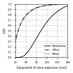
It is obvious Residential produced much worse time equivalence results comparing to the other two, primarily due to higher fuel load density.

Comparing agsint Kirby et al

Time equivalence CDF obtained from Kirby et al is shown in below.

print_df(kirby)

	Residential	Office	Retail
teq
30	0.169	0.464	0.404
45	0.193	0.647	NaN
60	0.361	0.800	0.734
75	0.629	0.896	NaN
90	0.844	0.928	0.912
105	0.953	0.973	NaN
120	0.991	0.982	0.968

fig, axes = plt.subplots(nrows=1, ncols=3, figsize=(2.1*3, 2.5), sharex=True, sharey=True, dpi=100)

for i, case in enumerate(cases_to_run):
    ax = axes[i]
    ax.scatter(kirby.index.values, kirby[case].values, label='Kirby et al', marker='o', facecolors='none', edgecolors='k', linewidths=.8)
    ax.plot(kirby.index.values[~np.isnan(kirby[case].values)], kirby[case].values[~np.isnan(kirby[case].values)], ls='--', c='k', lw=.5)
    ax.scatter(kirby.index.values, dict_func_teq2cdf[case](kirby.index.values), label='SFEPRAPY', marker='^', facecolors='none', edgecolors='k', linewidths=.8)
    ax.plot(kirby.index.values, dict_func_teq2cdf[case](kirby.index.values), ls='-.', c='k', lw=.5)
    format_ax(ax=ax, xlabel='Equivalent of time exposure [$min$]', xlabel_fontsize='x-small', xticks=np.arange(30, 121, 30), xticks_minor=np.arange(30, 121, 15), ylim=(0, 1), yticks=np.arange(0, 1.1, 0.1), legend_title=case, legend_loc=4, legend_fontsize='xx-small', legend_title_fontsize='xx-small')
axes[0].set_ylabel('CDF', fontsize='x-small')

savefig(fig, 'benchmark_1.png')

end

MCS2: Monte Carlo Simulation Method 2 ASFE21 Part 2: Failure Probability Based Approach