ASFE21 Part 2: Failure Probability Based Approach¶

Part 1 of the analysis carried out for the conference paper submitted to ASFE21, “An Improved Reliability-Based Approach to Sepcifying Fire Resistance Periods For Buildings in England”

2021 May, Ian F.

Structural failure probability¶

Prepare MCS inputs¶

[5]:

print_df(df_inputs_2)

	Residential	Office	Retail
case_name
n_simulations	10000	10000	10000
fire_time_step	10	10	10
fire_time_duration	18000	18000	18000
fire_hrr_density:dist	uniform_	uniform_	uniform_
fire_hrr_density:lbound	0.32	0.15	0.27
fire_hrr_density:ubound	0.57	0.65	1.0
fire_load_density:dist	gumbel_r_	gumbel_r_	gumbel_r_
fire_load_density:lbound	10	10	10.0
fire_load_density:ubound	1200	1200	2000.0
fire_load_density:mean	780	420	600.0
fire_load_density:sd	234	126	180.0
fire_spread_speed:dist	uniform_	uniform_	uniform_
fire_spread_speed:lbound	0.0035	0.0035	0.0035
fire_spread_speed:ubound	0.019	0.019	0.019
fire_nft_limit:dist	norm_	norm_	norm_
fire_nft_limit:lbound	623.15	623.15	623.15
fire_nft_limit:ubound	1473.15	1473.15	1473.15
fire_nft_limit:mean	1323.15	1323.15	1323.15
fire_nft_limit:sd	93	93	93
fire_combustion_efficiency:dist	uniform_	uniform_	uniform_
fire_combustion_efficiency:lbound	0.8	0.8	0.8
fire_combustion_efficiency:ubound	1.0	1.0	1.0
window_open_fraction:dist	lognorm_mod_	lognorm_mod_	lognorm_mod_
window_open_fraction:ubound	0.9999	0.9999	0.9999
window_open_fraction:lbound	0.0001	0.0001	0.0001
window_open_fraction:mean	0.2	0.2	0.2
window_open_fraction:sd	0.2	0.2	0.2
phi_teq:dist	lognorm_	lognorm_	lognorm_
phi_teq:mean	1	1	1
phi_teq:sd	0.25	0.25	0.25
phi_teq:ubound	3	3	3
phi_teq:lbound	0.0001	0.0001	0.0001
beam_cross_section_area	0.017	0.017	0.017
beam_position_vertical	3.2	3.2	3.2
beam_rho	7850	7850	7850
fire_mode	3	3	3
fire_gamma_fi_q	1	1	1
fire_t_alpha	300	300	300
fire_tlim	0.333	0.333	0.333
protection_c	1700	1700	1700
protection_k	0.2	0.2	0.2
protection_protected_perimeter	2.14	2.14	2.14
protection_rho	800	800	800
room_height:dist	constant_	uniform_	constant_
room_height:lbound	2.4	2.8	4.5
room_height:ubound	2.4	4.5	7.0
room_wall_thermal_inertia	720	720	720
solver_temperature_goal	893.15	893.15	893.15
solver_max_iter	20	20	20
solver_thickness_lbound	0.0001	0.0001	0.0001
solver_thickness_ubound	0.045	0.045	0.045
solver_tol	1.0	1.0	1.0
window_open_fraction_permanent	0	0	0
timber_exposed_area	0	0	0
timber_charring_rate	0.7	0.7	0.7
timber_hc	13.2	13.2	13.2
timber_density	400	400	400
timber_solver_ilim	20	20	20
timber_solver_tol	1	1	1
beam_position_horizontal_ratio:dist	uniform_	uniform_	uniform_
beam_position_horizontal_ratio:lbound	0.6	0.6	0.6
beam_position_horizontal_ratio:ubound	0.9	0.9	0.9
room_floor_area:dist	uniform_	uniform_	constant_
room_floor_area:lbound	9.0	50.0	400.0
room_floor_area:ubound	30.0	1000.0	400.0
room_breadth_depth_ratio:dist	uniform_	uniform_	uniform_
room_breadth_depth_ratio:lbound	0.4	0.4	0.4
room_breadth_depth_ratio:ubound	0.6	0.6	0.6
window_height_room_height_ratio:dist	uniform_	uniform_	uniform_
window_height_room_height_ratio:lbound	0.3	0.3	0.5
window_height_room_height_ratio:ubound	0.9	0.9	1.0
window_area_floor_ratio:dist	uniform_	uniform_	uniform_
window_area_floor_ratio:lbound	0.05	0.05	0.05
window_area_floor_ratio:ubound	0.2	0.4	0.4

Run MCS¶

[6]:

# Run MCS
cases_to_run=['Residential', 'Office', 'Retail']
mcs = MCS2(print_stats=False)
mcs.inputs = df_inputs_2
mcs.n_threads = 6
mcs.run_mcs(cases_to_run=cases_to_run)

CASE                    : Residential
NO. OF THREADS          : 6
NO. OF SIMULATIONS      : 10000

100%|███████████████| 10000/10000 [00:05<00:00, 1968.03it/s]

CASE                    : Office
NO. OF THREADS          : 6
NO. OF SIMULATIONS      : 10000

100%|███████████████| 10000/10000 [00:04<00:00, 2452.21it/s]

CASE                    : Retail
NO. OF THREADS          : 6
NO. OF SIMULATIONS      : 10000

100%|███████████████| 10000/10000 [00:04<00:00, 2459.49it/s]

Time equivalence results¶

[8]:

fig, ax = plt.subplots(figsize=(2.5,2.5), dpi=100);
lss = ['-', '-.', 'dotted']
FRs = np.linspace(30, 180, 100)
for i, case in enumerate(cases_to_run):
    ax.plot(FRs, dict_func_teq2cdf[case](FRs), label=case, ls=lss[i], c='k')
format_ax(ax=ax, xlabel='Equivalent of time exposure, $x$ [$min$]', xlabel_fontsize='x-small', xlim=(30, 180), ylabel=r'CDF or $P(t_{eq,i}\leq x)$', ylim=(0, 1), xticks=np.arange(30, 181, 15,), yticks=np.arange(0, 1.1, 0.1))

savefig(fig, 'teq_2.png')

../../_images/user_guide_mcs2_asfe21_02_11_0.png

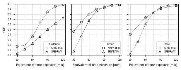
Comparing against Kirby et al¶

[9]:

kirby = pd.concat([
    pd.DataFrame({'Residential': [0.169, 0.193, 0.361, 0.629, 0.844, 0.953, 0.991]}, index=[30, 45, 60, 75, 90, 105, 120]),
    pd.DataFrame({'Office':      [0.464, 0.647, 0.800, 0.896, 0.928, 0.973, 0.982]}, index=[30, 45, 60, 75, 90, 105, 120]),
    pd.DataFrame({'Retail':      [0.404,        0.734,        0.912,        0.968]}, index=[30,     60,     90,      120]),
], axis=1)
kirby.index.name = 'teq'

# Compare against Kirby
fig, axes = plt.subplots(nrows=1, ncols=3, figsize=(2.1*3, 2.5), sharex=True, sharey=True, dpi=100)

for i, case in enumerate(cases_to_run):
    ax = axes[i]
    ax.scatter(kirby.index.values, kirby[case].values, label='Kirby et al', marker='o', facecolors='none', edgecolors='k', linewidths=.8)
    ax.plot(kirby.index.values[~np.isnan(kirby[case].values)], kirby[case].values[~np.isnan(kirby[case].values)], ls='--', c='k', lw=.5)
    ax.scatter(kirby.index.values, dict_func_teq2cdf[case](kirby.index.values), label='SFEPRAPY', marker='^', facecolors='none', edgecolors='k', linewidths=.8)
    ax.plot(kirby.index.values, dict_func_teq2cdf[case](kirby.index.values), ls='-.', c='k', lw=.5)
    format_ax(ax=ax, xlabel='Equivalent of time exposure [$min$]', xlabel_fontsize='x-small', xticks=np.arange(30, 121, 30), xticks_minor=np.arange(30, 121, 15), ylim=(0, 1), yticks=np.arange(0, 1.1, 0.1), legend_title=case, legend_loc=4, legend_fontsize='xx-small', legend_title_fontsize='xx-small')
axes[0].set_ylabel('CDF', fontsize='x-small')

savefig(fig, 'benchmark_2.png')

../../_images/user_guide_mcs2_asfe21_02_13_0.png

\(P_{f,fi}\) Failure probabilies due to structurally signification fire¶

[10]:

dict_p_i = {
    "Residential": dict(p_1=6.5e-7, p_2=0.2, p_3=0.0625, p_4=1),
    "Office": dict(p_1=3.0e-7, p_2=0.2, p_3=0.25, p_4=1),
    "Retail": dict(p_1=4.0e-7, p_2=0.2, p_3=0.25, p_4=1),
}

fig, axes = plt.subplots(nrows=1, ncols=3, figsize=(2.3*3, 2.5), sharex=True, sharey=True, dpi=100)
lss = ['-', (0, (5, 1)), '--', '-.', (0, (3, 1, 1, 1)), ':', (0, (5, 10))]
for i, case in enumerate(dict_teq.keys()):
    ax = axes[i]
    t = np.linspace(0, 180, 200)  # x-axis, time
    P_f_fi = 1 - dict_func_teq2cdf[case](t)  # failure probability due to structurally significant fires
    p_fi = np.prod(list(dict_p_i[case].values()))  # probability of structural significant fire occurance

    S_and_A = ((4, 800), (15, 800), (4, 1600), (15, 1600)) if case == 'Residential' else ((4, 1000), (15, 1000), (4, 2000), (15, 2000))

    for j, (S_, A_) in enumerate(S_and_A):
        ax.plot(t, p_fi * P_f_fi * (S_ * A_), label=f'S={S_:.0f}, $A_i$={A_*1e-3:.0f}k $m^2$', c='k', ls=lss[j], lw=1)
    format_ax(ax=ax, xlabel='Equivalent of time exposure [$min$]', xlim=(30, 180), xticks=np.arange(30, 181, 15), yscale='log', legend_title=case, legend_ncol=1, legend_loc=3, legend_fontsize='xx-small', legend_borderpad=0.1, legend_labelspacing=0.1)

ax = axes[0]
ax.set_ylabel('$P_{f,fi}$, failure probability due to\nstructurally significant fire [${year}^{-1}$]', fontsize='x-small')

savefig(fig, 'P_f_fi_vs_A.png')

../../_images/user_guide_mcs2_asfe21_02_15_0.png

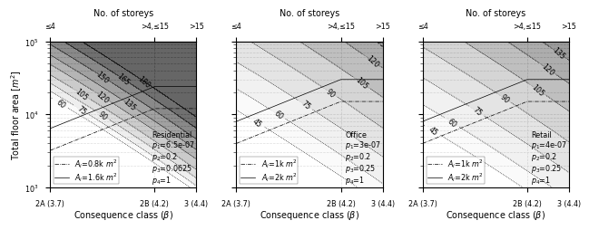
Recommended fire resistance periods¶

Buildings without sprinklers¶

[37]:

# visualisation, logscale
teqs = teqs_no_sprinklers
dict_p_i = dict_p_i_no_sprinklers
fig, axes = plt.subplots(figsize=(2.2*3, 2.65), nrows=1, ncols=3, dpi=100, sharex=True, sharey=True)

# plot no sprinklers
for i, key in enumerate(teqs):
    levels = np.arange(60, 181, 15) if key == 'Residential' else np.arange(45, 181, 15)
    ax = axes[i]
    ax.set_yscale('log')

    # add line text
    if key == 'Residential':
        ax.plot([3.7, 4.2, 4.4], [j*800 for j in [4, 15, 15]], c='k', lw=.5, ls='-.', label='$A_i$=0.8k $m^2$')
        ax.plot([3.7, 4.2, 4.4], [j*1600 for j in [4, 15, 15]], c='k', lw=.5, ls='-', label='$A_i$=1.6k $m^2$')
    elif key == 'Office':
        ax.plot([3.7, 4.2, 4.4], [j*1000 for j in [4, 15, 15]], c='k', lw=.5, ls='-.', label='$A_i$=1k $m^2$')
        ax.plot([3.7, 4.2, 4.4], [j*2000 for j in [4, 15, 15]], c='k', lw=.5, ls='-', label='$A_i$=2k $m^2$')
    elif key == 'Retail':
        ax.plot([3.7, 4.2, 4.4], [j*1000 for j in [4, 15, 15]], c='k', lw=.5, ls='-.', label='$A_i$=1k $m^2$')
        ax.plot([3.7, 4.2, 4.4], [j*2000 for j in [4, 15, 15]], c='k', lw=.5, ls='-', label='$A_i$=2k $m^2$')

    # clabel locations, i.e. clabel_manual
    if key == 'Residential':
        teq_and_beta = ((60, 3.75), (75, 3.85), (90, 3.95), (105, 3.85), (120, 3.95), (135, 4.08), (150, 3.95), (165, 4.05), (180, 4.15))
    elif key == 'Office':
        teq_and_beta = ((45, 3.80), (60, 3.90), (75, 4.03), (90, 4.15), (105, 4.30), (120, 4.35), (135, 4.36))
    elif key == 'Retail':
        teq_and_beta = ((45, 3.75), (60, 3.84), (75, 3.96), (90, 4.09), (105, 4.25), (120, 4.30), (135, 4.35))
    clabel_manual = list()
    for teq_, beta_ in teq_and_beta:
        aa = stats.norm(loc=0, scale=1).cdf(-beta_)
        bb = np.prod(list(dict_p_i[key].values())) * (1 - dict_func_teq2cdf[key](teq_))
        clabel_manual.append((beta_, aa/bb))

    cf = plot_contour(
        ax=ax, xx=beta, yy=area, zz=teqs[key], xlabel = r'Consequence class ($\beta$)', xlabel_fontsize='xx-small', levels=levels,
        xticks=[3.7, 4.2, 4.4], xticklabels=['2A (3.7)', '2B (4.2)', '3 (4.4)'], ticks_labelsize='xx-small',
        legend_visible=True, legend_loc='lower left', legend_borderpad=0.1, legend_labelspacing=.1, clabel_manual=clabel_manual
    )
    ax.set_axisbelow(True)
    ax.set_xlabel(r'Consequence class ($\beta$)', fontsize='x-small', labelpad=1)

    plot_contour_text_p_i(ax=ax, title=key, p_i=dict_p_i[key], ha='right', va='bottom', x=0.99, y=0.01, bbox_pad=0.4, bbox_fc=(0,0,0,0), linespacing=1.)

    ax2 = ax.secondary_xaxis('top')
    ax2.set_xlabel('No. of storeys', fontsize='x-small', labelpad=5)
    ax2.tick_params(labelsize='xx-small')
    ax2.set_xticks([3.7, 4.2, 4.4])
    ax2.set_xticklabels(['≤4', '>4,≤15', '>15'])


axes[0].set_ylabel('Total floor area [$m^2$]', fontsize='x-small', labelpad=1)

savefig(fig, 'contour_1_logscale.png')

../../_images/user_guide_mcs2_asfe21_02_19_0.png

Buildings with sprinklers¶

[34]:

# visualisation, logscale
teqs = teqs_sprinklers
dict_p_i = dict_p_i_sprinklers
fig, axes = plt.subplots(figsize=(2.2*3, 2.65), nrows=1, ncols=3, dpi=100, sharex=True, sharey=True)
for i, key in enumerate(teqs):
    levels = np.arange(60, 181, 15) if key == 'Residential' else np.arange(45, 181, 15)
    ax = axes[i]
    ax.set_yscale('log')

    # add line text
    if key == 'Residential':
        ax.plot([3.7, 4.2, 4.4], [j*800 for j in [4, 15, 15]], c='k', lw=.5, ls='-.', label='$A_i$=0.8k $m^2$')
        ax.plot([3.7, 4.2, 4.4], [j*1600 for j in [4, 15, 15]], c='k', lw=.5, ls='-', label='$A_i$=1.6k $m^2$')
    elif key == 'Office':
        ax.plot([3.7, 4.2, 4.4], [j*1000 for j in [4, 15, 15]], c='k', lw=.5, ls='-.', label='$A_i$=1k $m^2$')
        ax.plot([3.7, 4.2, 4.4], [j*2000 for j in [4, 15, 15]], c='k', lw=.5, ls='-', label='$A_i$=2k $m^2$')
    elif key == 'Retail':
        ax.plot([3.7, 4.2, 4.4], [j*1000 for j in [4, 15, 15]], c='k', lw=.5, ls='-.', label='$A_i$=1k $m^2$')
        ax.plot([3.7, 4.2, 4.4], [j*2000 for j in [4, 15, 15]], c='k', lw=.5, ls='-', label='$A_i$=2k $m^2$')

    # clabel locations, i.e. clabel_manual
    if key == 'Residential':
        teq_and_beta = ((60, 3.9), (75, 4.0), (90, 4.1), (105, 4.2), (120, 4.3), (135, 4.25), (150, 4.35), (165, 4.37))
    else:
        teq_and_beta = ((45, 4.02), (60, 4.12), (75, 4.23), (90, 4.35))
    clabel_manual = list()
    for teq_, beta_ in teq_and_beta:
        aa = stats.norm(loc=0, scale=1).cdf(-beta_)
        bb = np.prod(list(dict_p_i[key].values())) * (1 - dict_func_teq2cdf[key](teq_))
        clabel_manual.append((beta_, aa/bb))

    cf = plot_contour(
        ax=ax, xx=beta, yy=area, zz=teqs[key], xlabel = r'Consequence class ($\beta$)', xlabel_fontsize='xx-small', levels=levels,
        xticks=[3.7, 4.2, 4.4], xticklabels=['2A (3.7)', '2B (4.2)', '3 (4.4)'], ticks_labelsize='xx-small',
        legend_visible=True, legend_loc='lower left', legend_borderpad=0.1, legend_labelspacing=.1,
        clabel_manual=clabel_manual
    )
    ax.set_axisbelow(True)
    ax.set_xlabel(r'Consequence class ($\beta$)', fontsize='x-small', labelpad=1)

    plot_contour_text_p_i(ax=ax, title=key, p_i=dict_p_i[key], ha='right', va='bottom', x=0.99, y=0.01, bbox_pad=0.4, bbox_fc=(0,0,0,0), linespacing=1.0)

    ax2 = ax.secondary_xaxis('top')
    ax2.set_xlabel('No. of storeys', fontsize='x-small', labelpad=5)
    ax2.tick_params(labelsize='xx-small')
    ax2.set_xticks([3.7, 4.2, 4.4])
    ax2.set_xticklabels(['≤4', '>4,≤15', '>15'])

axes[0].set_ylabel('Total floor area [$m^2$]', fontsize='x-small', labelpad=1)
axes[0].set_yscale('log')

savefig(fig, 'contour_2_logscale.png')

../../_images/user_guide_mcs2_asfe21_02_23_0.png

Comparing against BS 9999:2017¶

[18]:

print_df(results)

	Method	Occupancy	Sprinkler	A [m²]	>5, ≤18 m	>18, ≤30 m	>30 m	100 m
0	BS 9999	Residential	False	NaN	60.0	90.0	120.0	120.0
1	SFEPRAPY	Residential	False	800.0	60.0	165.0	195.0	225.0
2	SFEPRAPY	Residential	False	1600.0	60.0	195.0	225.0	255.0
3	BS 9999	Residential	True	NaN	60.0	60.0	120.0	120.0
4	SFEPRAPY	Residential	True	800.0	60.0	60.0	90.0	120.0
5	SFEPRAPY	Residential	True	1600.0	60.0	75.0	120.0	150.0
6	BS 9999	Office	False	NaN	60.0	90.0	120.0	120.0
7	SFEPRAPY	Office	False	1000.0	45.0	90.0	105.0	120.0
8	SFEPRAPY	Office	False	2000.0	45.0	105.0	120.0	135.0
9	BS 9999	Office	True	NaN	30.0	60.0	120.0	120.0
10	SFEPRAPY	Office	True	1000.0	45.0	45.0	60.0	75.0
11	SFEPRAPY	Office	True	2000.0	45.0	60.0	75.0	90.0
12	BS 9999	Retail	False	NaN	60.0	90.0	120.0	120.0
13	SFEPRAPY	Retail	False	1000.0	45.0	105.0	120.0	135.0
14	SFEPRAPY	Retail	False	2000.0	60.0	120.0	135.0	150.0
15	BS 9999	Retail	True	NaN	60.0	60.0	120.0	120.0
16	SFEPRAPY	Retail	True	1000.0	45.0	60.0	75.0	90.0
17	SFEPRAPY	Retail	True	2000.0	45.0	75.0	90.0	105.0

end

ASFE21 Part 1: Time equivalence Useful Notebooks